The pendulum and the three magnets
Fractals are generally presented as mathematical curiosities, but their discovery came from very practical engineering considerations in the study of practical system. Here is a popular example of a very real physical system that can produce a beautiful fractal : the pendulum and the three magnets.
In this setup, illustrated below, a solid made of iron hangs from a thread over three magnets. Like a simple pendulum, when left to run from a starting position, it will swing back and forth until coming to a rest. But due to the magnets’ pull, the pendulum will eventually stop at a rest position near one of the three magnets instead of directly below its attach point.

What is not obvious from the start is where the pendulum will end – which magnet will it pick ? We can code a simulation to try to see what kind of trajectories the pendulum follows as it swings. Let’s start by a little physics. First, we list forces are acting upon the pendulum: gravity, the magnetic pull of each magnet, and friction.
Gravity is not a harsh mistress
Like a good physicist, we will make a couple of simplifying assumptions: we will only consider the position p of the pendulum in the horizontal plane. The mass m of the pendulum is 1 and the acceleration of gravity g = 1. We’re only here to see the behavior of the system, not make any accurate prediction. While we’re at it, we make the usual assumption that the pendulum swings at small angles. This simplifies the expression of the gravitational force to
\mathbf{F_G} = - {\mathbf{p}}Intuitively, gravity will pull back the pendulum towards the center, which is what we want. Let’s move on
Magnets, how do they work ?
If we were to model magnets as single magnetic charges the force between them would be proportional to the inverse squared distance between them (1/r2) but it turns out that more accurate models of magnetic dipoles give a law proportional to (1/r4) instead, so the magnetic force for magnet at position m will be directed from p to m
\mathbf{F_M} = \frac{K} {||\vec{PM}||^4} \cdot \frac{\vec{PM}} {||\vec{PM}||} = K \frac{\vec{PM}} {||\vec{PM}||^5}\;,where K is a constant hiding all the unwieldy magnetic-related terms (like the permissivity of vacuum and the strength of the magnets). We can choose it in the simulation to make the effect of the magnets stronger or weaker relative to gravity.
In real life the expression for the magnetic force change as the magnets get close to each other (it does not become infinite if the magnets stick). We don’t want to model this or have infinite values, so we add use an extra term h2 which will represent the “height” of the pendulum above the magnets.
Time to simulate
Friction will simply be a damping term on the velocity. We now turn to the bread and butter of physics simulation: the semi-implicit Euler method, which discretizes the equations of motion with a fixed time step dt.
Let’s try in python.
def update(pos, vel, dt):

    # Gravitational force
    gravity =  -p

    # Magnetic force
    magnets = np.zeros(2)
    for magnet_p in magnet_positions:
        diff = magnet_p - pos
        d2 = diff.dot(diff)
        v = K / ((d2 + h*h)**(5/2))

        magnets += v * diff


    # Semi implicit euler : first update velocity
    vel += dt * (gravity + magnets)
    vel *= (1.0 - dt * friction)
    # Then update position
    pos += dt * vel

    return pos,vel
Now we simply let go our pendulum from a starting position with a velocity of 0 and call update() until the velocity reaches a small enough value (say 0.001). We can plot the trajectory on the 2D plane, which yields some interesting curves :


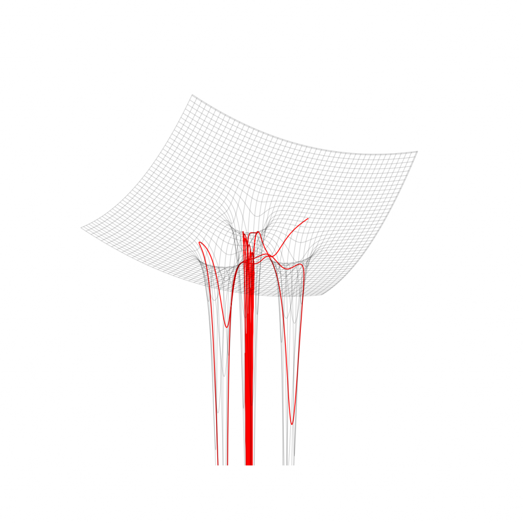
In both cases, the pendulum swings around each of the magnets before settling on one of them. Each magnet is (quite literally in this case) an attractor for the pendulum system, as they are the only stable equilibrium points. The equilibrium point is in fact slightly off of the magnet position, where the magnetic force and gravity balance each other. This becomes quite obvious when visualizing the potential field associated with the gravitational and magnetic forces, here shown with one of the trajectories drawn above.
That’s Chaos Theory
A more interesting property is that the system is highly sensitive to initial conditions: even when starting from very close points, we get very different trajectories.
This sensitivity to initial condition is the hallmark of chaos theory, and behind every chaotic system there is a beautiful fractal (and sometimes a T-rex)

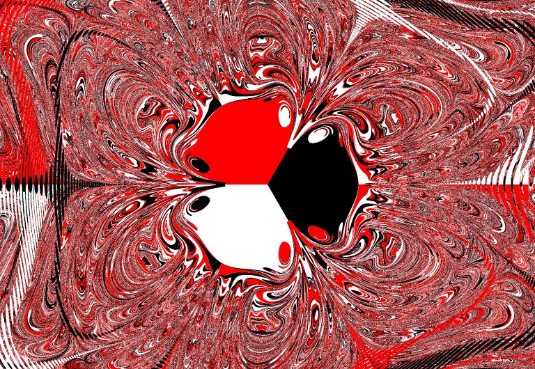
We can make this fractal appear by drawing the attractor basins of each magnet. We simulate the pendulum’s trajectory from every starting position on a 2D grid and color each pixel according to which of the three magnets it settles on.
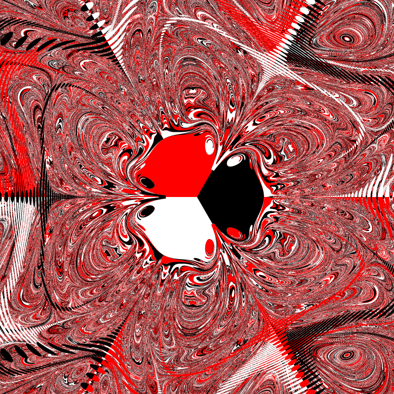
This makes the symmetry of the problem quite obvious! The three big plain-colored zones in the middle are the areas where the pendulum starts close to one of the magnets and simply swings back towards it without visiting any other. But anywhere else, the beautiful chaotic nature of the problem appears. We can see that sensitivity by looking at how rapidly the colors alternate : by moving from one pixel to the next (about a 0.002 difference in position) the pendulum ends up on a different rest state.
Like every fractal this one does has very fine detail. Let’s zoom closer until we reach the simulation precision.
Expect more animations coming up when I write a GPU implementation. In the meantime you can peruse the C++ code on github
Links
Some other pages about this fractal from which I’ve drawn inspiration:
- Chaos In the Magnetic pendulum, Institute of Mathematics and its Applications.
- The Magnetic Pendulum, Chalkdust Magazine
- Le Pendule et les trois aimants, Christophe Jacquet